A Tip for using Excel to Validate HDL templates
HCM Data Loader (HDL) data ready to load into Oracle HCM Cloud is in pipe separated text file format, however most people will create and manipulate these files in MS Excel as it’s the handy swiss-army-knife for data manipulation that almost everyone is familiar with.
The way that we’ve worked is that we create template files containing the sheets and columns corresponding to the fields that the client is using, which the client then populates, then we’ll validate and load into HCM Cloud. Although we use the Data File Validator for HDL as a final pass, most of this validation is first performed in Excel.
Some of this validation is basic (checking for trailing spaces, making sure the provided values are valid in the lookups etc) and some is slightly more complex, eg. looking at consistency across templates. It was whilst doing the latter today that I colleague and I came across a tip that we didn’t previously know.
How VLOOKUP almost works
My normal method of looking up a value in a table elsewhere in Excel is to use the VLOOKUP function. It’s quick, easy and has saved us from countless data issues by spotting problems early. There’s a problem however, which I’ll explain, and provide the solution.
A simplified example is Banks and Branches. First we obtain the list of valid Banks, then we check the list of Bank Branches to make sure that the Bank operating each Branch appears on our list of Banks.
On the left here we have the list of valid Banks in column B, and a text string in column C saying ‘OK’. This is the value that gets returned if the bank matches. (This is a heavily simplified example, the genuine data would have many thousands of branches to check.)
On the right we have the list of Branch owners to lookup against the list on the left.

By using a formula we want to check each of the banks in column E is somewhere in the table on the left. So we use:
=vlookup(<bank to check>, <table of valid banks>, <column to return>, FALSE)
which translates to this for the first cell:
=vlookup(e3,$b$3:$c$8,2,FALSE)
This works a treat, giving the following results:
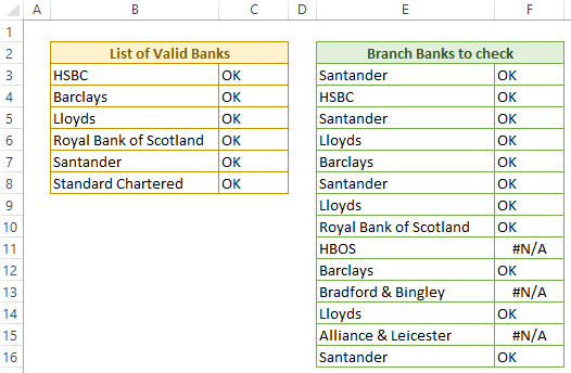
We can clearly see which branches are run by banks on our list and which are not.
The reason that this sometimes fails is VLOOKUP isn’t case sensitive. Looking up the value LLoyds in the valid banks table would result in a match (despite the second upper case L), however it would obviously fail when we tried to load the data in using HDL.

The Solution
The method that I now use is a ‘Lookup Exact’. It combines two Excel functions (surprisingly, LOOKUP and EXACT) to give a case sensitive equivalent to VLOOKUP (with the added benefit that the lookup table doesn’t need to be sorted alphabetically).
The formula has the syntax:
=LOOKUP(1,1/EXACT(<table of valid banks>, <bank to check>), <values to return>)
which translates to this for the first cell:
=LOOKUP(1,1/EXACT($B$3:$B$8,E3),$C$3:$C$8)
And if I add this to column G we can see that it looks up perfectly against our table, correctly identifying even those in the wrong case (where vlookup in column F fails us).

To give credit where due, I didn’t create this Excel function. It is well explained in this YouTube video:
